numpy实现多项式回归模型

前言

书接上回，上回我们介绍了线性回归，这次我们来关注一下多项式回归。

对于多项式回归，回归函数是回归变量多项式的回归 ，实际上线性回归是多项式回归中的特殊情况，即此自变量的项次是一次。

原理

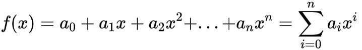
泰勒公式告诉我们，任何函数在一定区间内都可以用多项式函数进行逼近，即

假设我们的n=1，那么我们就回到了线性模型。

理论上我们的n越大，我们的函数就更加逼近原函数，不过在实际运算中，该值越大，计算量也就越大，而且计算机运算过程中也容易溢出，因此该值应该有一个比较符合实际意义的值。

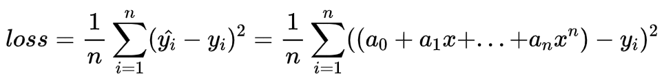
参照上文，我们可以写出损失函数为：

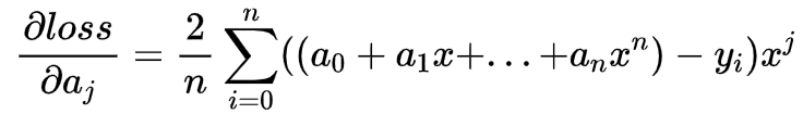
该函数对每一项的系数求导为：

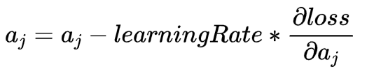
更新参数方法依旧是使用梯度下降分析法：

代码实现

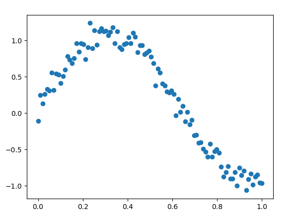
我们先产生一个三角函数的数据，并加入随机偏差，模拟非线性数据：

def Data():
    x = np.linspace(0, 1, 100)
    y = np.sin(5 * x) + 0.1 + np.random.randn(len(x)) * 0.1
    return x, y

再定义参数初始化函数：

def init(len=5):
    """
    len 是多项式次数，该函数返回多项式的每一个系数
    """
    return np.random.randn(len) * 0.5

接下来就是我们的回归主体部分啦！

在这之前，我们来学习一下怎么使用NumPy来实现多项式计算：在NumPy中，如果我们要计算:

f(x) = a + b * x + c * x^2 + d * x^3

可以使用：

f = np.poly1d(theta)
f(x)

其中，theta是多项式系数，例如计算f(x)=0.7 * x^2+ 0.6 * x + 0.5在x=1.2的值，可以用下面的代码完成：

f = np.poly1d([0.7, 0.6, 0.5])
f(1.2)
2.2279999999999998

记住，np.poly1d()中的参数是从多项式最高项开始的

因此我们可以定义计算y_hat的函数：

def getY_Hat(x, theta):
    # 根据 theta 作为系数，生成多项式函数
    f = np.poly1d(theta)
    return f(x)

有了该函数后，我们可以继续定义loss函数：

def loss(y, yHat):
    n = len(y)
    t1 = (y - yHat) * (y - yHat)
    return sum(t1) / n

梯度下降分析法：

# 更新每一个参数
n = len(theta)
for j in range(n):
    sm = sum((y_hat - y) * (x ** (n - 1 - j)))
    roundThetaIdx =  2 * sm / n
    theta[j] = theta[j] - learning_rate * roundThetaIdx

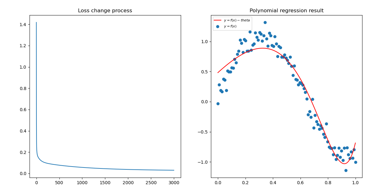
最终的结果：

完整代码

# -*- coding: utf-8 -*-
"""
Created on Tue Apr 12 17:47:32 2022

@author: YaleXin
"""
import numpy as np
import matplotlib.pyplot as plt 

#%%
def Data():
    x = np.linspace(0, 1, 100)
    y = np.sin(5 * x) + 0.1 + np.random.randn(len(x)) * 0.1
    return x, y
#%%
def init(len=5):
    """
    len 是多项式次数
    """
    return np.random.randn(len) * 0.5
#%%
def getY_Hat(x, theta):
    # 根据 theta 作为系数，生成多项式函数
    f = np.poly1d(theta)
    return f(x)
#%%
def loss(y, yHat):
    n = len(y)
    t1 = (y - yHat) * (y - yHat)
    return sum(t1) / n
#%%
def PolynomialRegression(x, y, theta, ax, epoch=100, learning_rate = 0.01):
    """
    梯度下降法
    """
    ax.set_title("Loss change process")
    loss_x = []
    loss_y = []
    for i in range(epoch):

        y_hat = getY_Hat(x, theta)
        lst = loss(y, y_hat)
        loss_x.append(i)
        loss_y.append(lst)
        print("lost = " + str(lst))
        
        # 更新每一个参数
        n = len(theta)
        for j in range(n):
            sm = sum((y_hat - y) * (x ** (n - 1 - j)))
            roundThetaIdx =  2 * sm / n
            theta[j] = theta[j] - learning_rate * roundThetaIdx
    ax.plot(loss_x, loss_y)
    return theta
#%%

def plotAns(x, y, Y, ax):
    """绘制图形    
    y是数据原始的y值，Y是拟合得到的值
    """
    ax.set_title('Polynomial regression result')
    ax.scatter(x, y, label = r'$y = f(x)$')
    ax.plot(x, Y, label=r'$y = f(x)-theta $', color='red')
    ax.legend(loc='upper left',prop={'family':'SimHei','size':8})

#%%
if __name__ == "__main__":
    
    fig = plt.figure()
    cost_ax = fig.add_subplot(1,2,1)  
    ans_ax = fig.add_subplot(1,2,2)  
    
    # 载入多项式回归数据
    x, y = Data()
    
    # 初始化 最高次数为 10 的一组系数
    theta = init(10)

    # 设置学习率
    my_learning_rate = 0.02
    
    # # 求解最优参数
    theta = PolynomialRegression(x, y, theta, cost_ax,epoch=3000)
    f = np.poly1d(theta)
    yhat = f(x)
    
    plotAns(x, y, yhat, ans_ax)
    plt.show()